Activation Functions

Sigmoid

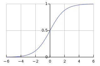
Range: (0, 1)
Formula: $f(x) = \frac{1}{1 + e^{-x}} = \frac{e^x}{e^x + 1} = 1 - f(-x)$
Derivative: $f'(x) = f(x)(1 - f(x))$
Use: Output layer of a binary classification model.
Issue: Vanishing gradient problem.

Softmax

The softmax function takes as input a vector z of K real numbers, and normalizes it into a probability distribution consisting of K probabilities proportional to the exponentials of the input numbers.
prior to applying softmax, some vector components could be negative, or greater than one; and might not sum to 1;
but after applying softmax, each component will be in the interval (0,1) and the components will add up to 1.
For example,
- consider the following vector of logits: $z = [2.0, 1.0, 8.0]$
- Applying the softmax function to this vector yields the following probabilities: $\text{softmax}(z) = [0.002, 0.001, 0.997]$
Equation:

\[\text{softmax}(z)_i = \frac{e^{z_i}}{\sum_{j=1}^{K} e^{z_j}}\]
In our example:

\[\text{softmax}(z)_1 = \frac{e^{2.0}}{e^{2.0} + e^{1.0} + e^{8.0}} = 0.002\]

Tanh

Range: (-1, 1)
Formula: $f(x) = \frac{2}{1 + e^{-2x}} - 1$
Derivative: $f'(x) = 1 - f(x)^2$
Use: Hidden layers of a neural network.
Issue: Vanishing gradient problem.

ReLU (Rectified Linear Unit)

Range: [0, $\infty$)
Formula:

\[f(x) = x^+ = max(0, x) = \frac{x + |x|}{2} = \begin{cases} 0 & \text{if } x \leq 0 \\ x & \text{if } x > 0 \end{cases}\]
Derivative:

\[f'(x) = \begin{cases} 0 & \text{if } x < 0 \\ 1 & \text{if } x > 0 \end{cases}\]
Use: Hidden layers of a neural network.
Advantages
- Sparse activation: For example, in a randomly initialized network, only about 50% of hidden units are activated (have a non-zero output).
- Better gradient propagation: Fewer vanishing gradient problems compared to sigmoidal activation functions that saturate in both directions.
- Efficient computation: Only comparison, addition and multiplication.
Potential problems
- Non-differentiable at zero; however, it is differentiable anywhere else, and the value of the derivative at zero can be arbitrarily chosen to be 0 or 1.
- Not zero-centered.
- Unbounded.
- Dying ReLU problem:
  - Dying ReLU problem. Meaning that the neuron will never activate on any data point again if its weights are updated in such a way that the weighted sum of the neuron's input is negative for all data points in the training set.
  - ReLU (rectified linear unit) neurons can sometimes be pushed into states in which they become inactive for essentially all inputs. In this state, no gradients flow backward through the neuron, and so the neuron becomes stuck in a perpetually inactive state and "dies". This is a form of the vanishing gradient problem. In some cases, large numbers of neurons in a network can become stuck in dead states, effectively decreasing the model capacity. This problem typically arises when the learning rate is set too high. It may be mitigated by using leaky ReLUs instead, which assign a small positive slope for $x < 0$; however, the performance is reduced.
Variants: Leaky ReLU, Parametric ReLU, Exponential Linear Unit (ELU), Scaled Exponential Linear Unit (SELU), Swish, Mish.

Leaky ReLU

Leaky ReLUs allow a small, positive gradient when the unit is not active, helping to mitigate the vanishing gradient problem.

Formula:

\[f(x) = \begin{cases} 0.01x & \text{if } x \leq 0 \\ x & \text{if } x > 0 \end{cases}\]
Derivative:

\[f'(x) = \begin{cases} 0.01 & \text{if } x < 0 \\ 1 & \text{if } x > 0 \end{cases}\]

Parametric ReLU (PReLU)

making the coefficient of leakage into a parameter that is learned along with the other neural-network parameters.
Formula:

\[f(x) = \begin{cases} \alpha x & \text{if } x < 0 \\ x & \text{if } x \geq 0 \end{cases}\]

GELU (Gaussian Error Linear Unit)

It is utilized by BERT, GPT-2, ViT, and CLIP(some parts).
It is a smooth approximation to the rectifier.
- This non-convex, non-monotonic function is not linear in the positive domain and exhibits curvature at all points.
- Meanwhile ReLUs and ELUs, which are convex and monotonic activations, are linear in the positive domain and thereby can lack curvature
It is defined as:

\[GELU(x) = x . \Phi(x)\]

where $\Phi(x)$ is the cumulative distribution function of the standard normal distribution.
We can approximate GELU with the following formula:

\[GELU(x) = 0.5x(1 + \tanh(\sqrt{2/\pi}(x + 0.044715x^3)))\]

# GELU: As defined in GPT-2 Repository
import torch
import torch.nn.functional as F

def gelu(x):
    return 0.5*x*(1+tf.tanh(np.sqrt(2/np.pi)*(x+0.044715*tf.pow(x, 3))))

Advantages:

Smoothness: GELU is smooth everywhere, including around the origin. This smoothness can help in gradient-based optimization methods by providing continuous gradients, which can lead to more stable and efficient training.
Sigmoid-Like Behavior: GELU exhibits a sigmoid-like behavior, particularly for negative values. This can help mitigate issues like vanishing gradients commonly associated with activation functions like ReLU, especially for deep neural networks.
Saturation Handling: GELU saturates more smoothly compared to ReLU for large negative values. This property can prevent the gradient from becoming too small, thus addressing the vanishing gradient problem.
Performance: Empirical studies have shown that GELU sometimes outperforms traditional activation functions like ReLU and its variants on certain tasks and architectures. It has been observed to improve convergence speed and generalization performance in some scenarios.
Compatibility with Modern Hardware: While GELU involves more complex mathematical operations compared to ReLU, it is still computationally efficient and can be effectively implemented on modern hardware platforms, including GPUs and TPUs.

Cons:

Computational Complexity: GELU involves more complex mathematical operations compared to simpler activation functions like ReLU. This increased complexity can lead to slightly higher computational costs, although it's often manageable in practice.
Lack of Theoretical Justification: While empirical studies have shown the effectiveness of GELU in certain cases, its theoretical properties are not as well understood as some other activation functions. This can make it challenging to analyze the behavior of neural networks using GELU from a theoretical perspective.
Sensitivity to Hyperparameters: Like many other aspects of deep learning models, the performance of GELU can be sensitive to hyperparameters such as learning rate, initialization schemes, and model architecture. Finding optimal hyperparameters may require additional tuning effort.
Limited Empirical Evidence: While GELU has shown promising results in various applications, its superiority over other activation functions may not be consistent across all tasks and datasets. More empirical studies are needed to fully understand its strengths and limitations in different scenarios.

Paper: Gaussian Error Linear Units (GELUs)

Swish function ($Swish_{ \beta}$)

\[ Swish_{ \beta}(x) = x \cdot sigmoid(\beta x)\]

For Swish, the parameter $\beta$ can be adjusted to control the shape of the function.
$\beta$ was intended to added as learnable parameter, though researchers usually let β = 1 and do not use the learnable parameter.
For $\beta = 0$, it becomes $f(x) = 0.5x$.
For $\beta = 1$, it becomes SiLU (Sigmoid linear unit) $= x \cdot sigmoid(x)$
For $\beta$ → $\infty$, it becomes ReLU.
Thus, it can be viewed as a smoothing function which nonlinearly interpolates between a linear function and the ReLU function
In 2017, after performing analysis on ImageNet data, researchers from Google indicated that using this function as an activation function improves the performance, compared to ReLU and sigmoid functions.
It is believed that one reason for the improvement is that the swish function helps alleviate the vanishing gradient problem during backpropagation.

SiLU - Sigmoid Linear Unit ($Swish_{1}$)

\[ Swish_{ \beta = 1}(x) = x \cdot sigmoid(x)\]

SiLU is a smooth, non-monotonic activation function that is differentiable everywhere.
derivative of SiLU is given by:

\[Swish_{1}'(x) = x \cdot \sigma'(x) + \sigma(x)\]

where $\sigma(x)$ is the sigmoid function.

GLU (Gated Linear Unit)

Formula:

\[GLU(x, W, V, b, c) = \sigma(Wx + b) \odot (Vx + c)\]

where $\odot$ denotes element-wise multiplication, $\sigma$ is the sigmoid function, and $W$, $V$, $b$, and $c$ are learnable parameters.

We can also define GLU variants using other activation functions:

\[ReGLU(x, W, V, b, c) = ReLU(Wx + b) \odot (Vx + c)\]

\[GEGLU(x, W, V, b, c) = GELU(Wx + b) \odot (Vx + c)\]

\[SwiGLU(x, W, V, b, c, \beta) = Swish_{\beta}(Wx + b) \odot (Vx + c)\]

\[SwiGLU(x, W, V, b, c, 1) = Swish_{1}(Wx + b) \odot (Vx + c)\]

Papers:

Language Modeling with Gated Convolutional Networks
GLU Variants Improve Transformer. Mentions SwiGLU activation function.

SwiGLU Activation Function (Llama-2)

Note

SwiGLU is a combination of the Swish and GLU activation functions.
It is used in Llama-2 architecture.
Before we understand SwiGLU, we need to understand the GLU and Swish activation functions.
Refer to the GLU and Swish activation functions for more details.

As we know from the GLU activation function, SwiGLU is defined as:

\[SwiGLU(x, W, V, b, c, 1) = Swish_{1}(Wx + b) \odot (Vx + c)\]

To understand the SwiGLU activation function, it is best to learn with code. Here I will not only explain the SwiGLU activation function but also show how it is implemented in the FFN layer of the transformer architecture.

Let's try to define the FFN layer with SwiGLU activation function:

Recall the FFN layer in the transformer architecture. They used a two-layer feed-forward network with ReLU activation function in between. The output of the first layer is passed through the activation function(ReLU) and then to the second layer.

\[FFN(x) = W_{2} \cdot ReLU(W_{1} \cdot x + b_{1}) + b_{2}\]

Applying GLU with ReLU to the output of the first layer:

\[FFF_{ReGLU}(x) = W_{2} [ ReLU(W_{1} \cdot x + b_{1}) \odot (V \cdot x + c) ] + b_{2}\]

Finally, SwiGLU:

\[FFN_{SwiGLU}(x) = W_{2} [ Swish_{1}(W_{1} \cdot x + b_{1}) \odot (V \cdot x + c) ] + b_{2}\]

where W₁, V, and W₂ are learnable weight matrices.

SwiGLU: As in xformers (by Facebook Research)

import torch
import torch.nn as nn
import torch.nn.functional as F

class SwiGLU(nn.Module):
    def __init__(self, input_dim, hidden_dim, output_dim):
        super(SwiGLU, self).__init__()
        self.W1 = nn.Parameter(torch.randn(input_dim, hidden_dim))
        self.V = nn.Parameter(torch.randn(input_dim, hidden_dim))
        self.W2 = nn.Parameter(torch.randn(hidden_dim, output_dim))
        self.b1 = nn.Parameter(torch.randn(hidden_dim))
        self.c = nn.Parameter(torch.randn(hidden_dim))
        self.b2 = nn.Parameter(torch.randn(output_dim))

    def forward(self, x):
        x1 = F.linear(x, W1, b1)     # First layer. Will go through SiLU activation function.
        x2 = F.linear(x, V, c)      # GLU: Other matrix (right half of the GLU activation function)
        hidden = F.silu(x1) * x2    # GLU activation function.(lef)
        return F.linear(hidden, W2, b2) # Second layer of FFN.

        # Note: In xformers library, the authors used a different notation for the weight matrices and biases than the GLU paper.
        # Instead of w1,v, w2, they used w1, w2, w3.
        # Instead of b1, c, b2, they used b1, b2, b3.
        x1 = F.linear(x, w1, b1)
        x2 = F.linear(x, w2, b2)
        hidden = F.silu(x1) * x2
        return F.linear(hidden, w3, b3)

All of these layers have three weight matrices, as opposed to two for the original FFN.
In GLU papar, To keep the number of parameters and the amount of computation constant, they reduce the number of hidden units (the second dimension of W and V and the first dimension of W2) by a factor of 2/3 when comparing these layers to the original two-matrix version.

paper: GLU Variants Improve Transformer

Comparison of Activation Functions

Name	Function $g(x)$	Derivative of $g = g'(x)$	Range	Order of continuity
Logistic, sigmoid, or soft step	$\sigma(x) \approx \frac{1}{1 + e^{-x}}$	$g(x)(1 - g(x))$	$(0, 1)$	$C^{\infty}$
Hyperbolic tangent (tanh)	$\tanh(x) \approx \frac{e^x - e^{-x}}{e^x + e^{-x}}$	$1 - g(x)^2$	$(-1, 1)$	$C^{\infty}$
Rectified linear unit (ReLU)	$(x)^+ \approx \begin{cases} 0 & \text{if } x \leq 0 \\ x & \text{if } x > 0 \end{cases}$	$\begin{cases} 0 & \text{if } x < 0 \\ 1 & \text{if } x > 0 \end{cases}$	$[0, \infty)$	$C^{0}$
Gaussian Error Linear Unit (GELU)	$\frac{1}{2}x\left(1+\operatorname{erf}\left(\frac{x}{\sqrt{2}}\right)\right) \approx x\Phi(x)$	$\Phi(x) + x\phi(x)$	$(-0.17\ldots, \infty)$	$C^{\infty}$
Scaled exponential linear unit (SELU)	$\lambda \begin{cases} \alpha(e^x - 1) & \text{ if } x < 0 \\ x & \text{ if } x \geq 0 \end{cases}$ with parameters $\alpha = 1.67326$ and $\lambda = 1.0507$	$\lambda \begin{cases} \alpha e^x & \text{ if } x < 0 \\ 1 & \text{ if } x \geq 0 \end{cases}$	$(-\lambda \alpha, \infty)$	$C^{0}$
Leaky rectified linear unit (Leaky ReLU)	$\begin{cases} 0.01x & \text{if } x \leq 0 \\ x & \text{if } x > 0 \end{cases}$	$\begin{cases} 0.01 & \text{if } x < 0 \\ 1 & \text{if } x > 0 \end{cases}$	$(-\infty, \infty)$	$C^{0}$
Sigmoid linear unit (SiLU) / Swish	$swish(x) = x \cdot sigmoid( \beta x)$ For $\beta = 1$, it becomes SiLU $SiLU = \frac{x}{1 + e^{-x}}$	$\frac{1 + e^{-x} + xe^{-x}}{(1 + e^{-x})^2}$	$(-0.278\ldots, \infty)$	$C^{\infty}$

Other:

Name	Function $g(x)$	Derivative of $g = g'(x)$	Range	Order of continuity
Identity	$x$	$1$	$(-\infty, \infty)$	$C^{\infty}$
Binary step	$0$ if $x < 0$, $1$ if $x \geq 0$	$0$	$\{0, 1\}$	$C^{-1}$
Soboleva modified hyperbolic tangent	$\operatorname{smht}(x) \approx \frac{e^{ax} - e^{-bx}}{e^{cx} + e^{-dx}}$		$(-1, 1)$	$C^{\infty}$
Softplus	$\ln(1 + e^x)$	$\frac{1}{1 + e^{-x}}$	$(0, \infty)$	$C^{\infty}$
Exponential linear unit (ELU)	$\begin{cases} \alpha(e^x - 1) & \text{if } x \leq 0 \\ x & \text{if } x > 0 \end{cases}$ with parameter $\alpha$	$\begin{cases} \alpha e^x & \text{if } x < 0 \\ 1 & \text{if } x > 0 \end{cases}$	$(-\alpha, \infty)$	$C^{1}$ if $\alpha = 1$ else $C^{0}$
Parametric rectified linear unit (PReLU)	$\begin{cases} \alpha x & \text{if } x < 0 \\ x & \text{if } x \geq 0 \end{cases}$	$\begin{cases} \alpha & \text{if } x < 0 \\ 1 & \text{if } x \geq 0 \end{cases}$	$(-\infty, \infty)$	$C^{0}$
Gaussian	$e^{-x^2}$	$-2xe^{-x^2}$	$(0, 1]$	$C^{\infty}$

Monotonicity:

Monotonicity: An activation function is monotonic if it is either entirely non-increasing or non-decreasing.
For example, the ReLU activation function is non-decreasing for $x \geq 0$ and constant for $x < 0, making it a monotonic function. *
Non-monotonicity: An activation function is non-monotonic if it is neither entirely non-increasing nor non-decreasing.
For example, GLU (Gated Linear Unit), Swish function are non-monotonic activation functions.
Monotonic activation functions are preferred in some contexts because they ensure that the output of the function changes in the same direction as the input.
This property can simplify the optimization process and help avoid issues like oscillations or instability during training.

Name	Function \(g(x)\)	Derivative of \(g = g'(x)\)	Range	Order of continuity
Logistic, sigmoid, or soft step	\(\sigma(x) \approx \frac{1}{1 + e^{-x}}\)	\(g(x)(1 - g(x))\)	\((0, 1)\)	\(C^{\infty}\)
Hyperbolic tangent (tanh)	\(\tanh(x) \approx \frac{e^x - e^{-x}}{e^x + e^{-x}}\)	\(1 - g(x)^2\)	\((-1, 1)\)	\(C^{\infty}\)
Rectified linear unit (ReLU)	\((x)^+ \approx \begin{cases} 0 & \text{if } x \leq 0 \\ x & \text{if } x > 0 \end{cases}\)	\(\begin{cases} 0 & \text{if } x < 0 \\ 1 & \text{if } x > 0 \end{cases}\)	\([0, \infty)\)	\(C^{0}\)
Gaussian Error Linear Unit (GELU)	\(\frac{1}{2}x\left(1+\operatorname{erf}\left(\frac{x}{\sqrt{2}}\right)\right) \approx x\Phi(x)\)	\(\Phi(x) + x\phi(x)\)	\((-0.17\ldots, \infty)\)	\(C^{\infty}\)
Scaled exponential linear unit (SELU)	\(\lambda \begin{cases} \alpha(e^x - 1) & \text{ if } x < 0 \\ x & \text{ if } x \geq 0 \end{cases}\) with parameters \(\alpha = 1.67326\) and \(\lambda = 1.0507\)	\(\lambda \begin{cases} \alpha e^x & \text{ if } x < 0 \\ 1 & \text{ if } x \geq 0 \end{cases}\)	\((-\lambda \alpha, \infty)\)	\(C^{0}\)
Leaky rectified linear unit (Leaky ReLU)	\(\begin{cases} 0.01x & \text{if } x \leq 0 \\ x & \text{if } x > 0 \end{cases}\)	\(\begin{cases} 0.01 & \text{if } x < 0 \\ 1 & \text{if } x > 0 \end{cases}\)	\((-\infty, \infty)\)	\(C^{0}\)
Sigmoid linear unit (SiLU) / Swish	\(swish(x) = x \cdot sigmoid( \beta x)\) For \(\beta = 1\), it becomes SiLU \(SiLU = \frac{x}{1 + e^{-x}}\)	\(\frac{1 + e^{-x} + xe^{-x}}{(1 + e^{-x})^2}\)	\((-0.278\ldots, \infty)\)	\(C^{\infty}\)

Name	Function \(g(x)\)	Derivative of \(g = g'(x)\)	Range	Order of continuity
Identity	\(x\)	\(1\)	\((-\infty, \infty)\)	\(C^{\infty}\)
Binary step	\(0\) if \(x < 0\), \(1\) if \(x \geq 0\)	\(0\)	\(\{0, 1\}\)	\(C^{-1}\)
Soboleva modified hyperbolic tangent	\(\operatorname{smht}(x) \approx \frac{e^{ax} - e^{-bx}}{e^{cx} + e^{-dx}}\)		\((-1, 1)\)	\(C^{\infty}\)
Softplus	\(\ln(1 + e^x)\)	\(\frac{1}{1 + e^{-x}}\)	\((0, \infty)\)	\(C^{\infty}\)
Exponential linear unit (ELU)	\(\begin{cases} \alpha(e^x - 1) & \text{if } x \leq 0 \\ x & \text{if } x > 0 \end{cases}\) with parameter \(\alpha\)	\(\begin{cases} \alpha e^x & \text{if } x < 0 \\ 1 & \text{if } x > 0 \end{cases}\)	\((-\alpha, \infty)\)	\(C^{1}\) if \(\alpha = 1\) else \(C^{0}\)
Parametric rectified linear unit (PReLU)	\(\begin{cases} \alpha x & \text{if } x < 0 \\ x & \text{if } x \geq 0 \end{cases}\)	\(\begin{cases} \alpha & \text{if } x < 0 \\ 1 & \text{if } x \geq 0 \end{cases}\)	\((-\infty, \infty)\)	\(C^{0}\)
Gaussian	\(e^{-x^2}\)	\(-2xe^{-x^2}\)	\((0, 1]\)	\(C^{\infty}\)